resdb = DuckDBClient.of({
  sourcesink1: FileAttachment("sourcesink1.parquet"),
  sourcesink1_lookup: FileAttachment("sourcesink1_lookup.parquet"),
  sourcesink2: FileAttachment("sourcesink2.parquet"),
  sourcesink2_lookup: FileAttachment("sourcesink2_lookup.parquet")
  // sourcesink3: FileAttachment("sourcesink3.parquet"),
  // sourcesink3_lookup: FileAttachment("sourcesink3_lookup.parquet")
})Description
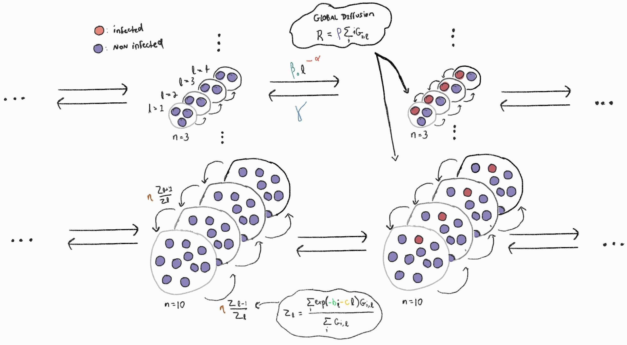
The key ingredients of the source-sink model1 are groups \(G\) of various size with a certain number of adopters \(i\) and of institution of level \(\ell\). We assume that with higher levels of institutional strength, \(\ell\), the institution will more effectively promote group-beneficial behavior, \(\ell\)\(\beta\). As it gets better, each adopter in the group also gain a collective benefit \(b\). But all of these toodily-doo perks are offset by an institutional implementation costs, \(c\), of entertaining larger groups. For instance, think of the process of unionization, promoting behaviors that are costly at individual level. When unionization becomes more successful, the unions can become ungaingly. Lastly adopters lose their behavioural trait at a rate \(\gamma\).
First master equation2:
\[\begin{align*} \frac{d}{dt}G_{i,\ell}^{diff} &= \ell \mathbin{\color{darkgreen}{\beta}} [(i-1) + R](n - i + 1)G_{i-1,\ell} \\ &- \ell\mathbin{\color{darkgreen}{\beta}} (i+R)(n-i) G_{i,\ell} \\ &+ \mathbin{\color{red}{\gamma}}(i+1)G_{i+1,\ell} - \mathbin{\color{red}{\gamma}} i G_{i,\ell} \end{align*}\]where \(R = \mathbin{\color{blue}{\rho}} \sum_{i',\ell'} i'G_{i',\ell'}\) represents the global diffusion of behaviors and primes denote variable over which we sum to calculate global quantity. The sum over adopters at each level weighted by global behavioural diffusion \(\rho\).
Second master equation:
\[\begin{align*} \frac{d}{dt}G_{i,\ell}^{select} &= \mathbin{\color{blue}{\rho}} [G_{i,\ell-1}(Z_\ell Z_{\ell-1}^{-1} + \mathbin{\color{midnightblue}{\mu}}) + G_{i,\ell+1}(Z\ell Z_{\ell + 1}^{-1} + \mathbin{\color{midnightblue}{\mu}})] \\ &-\mathbin{\color{blue}{\rho}}(Z_{\ell-1}Z_\ell^{-1} + Z_{\ell+1}^{-1} + 2\mathbin{\color{midnightblue}{\mu}})G_{i,\ell} \end{align*}\]where \(Z_\ell = \frac{\sum_{i'} exp(\mathbin{\color{seagreen}{b}}i'- \mathbin{\color{darkred}{c}}\ell)G_{i',\ell}}{\sum_{i'}G_{i',\ell}}\). Note that we add a constant rate of transition \(\mu\) to the selection proces.
Taken together we have the set of master equations:
\[ \frac{d}{dt}G_{i,\ell} = \frac{d}{dt}G_{i,\ell}^{diff} + \frac{d}{dt}G_{i,\ell}^{select} \]
Click to see the Julia code
function source_sink!(du, u, p, t)
    G, L, n = u, length(u.x), length(first(u.x))
    β, γ, ρ, b, c, μ = p
    Z, pop, R = zeros(L), zeros(L), 0.

    # Calculate mean-field coupling and observed fitness landscape
    for ℓ in 1:L
      n_adopt = collect(0:(n-1))
      Z[ℓ]    = sum(exp.(b*n_adopt .- c*(ℓ-1)) .* G.x[ℓ])
      pop[ℓ]  = sum(G.x[ℓ])
      R       += sum(ρ*n_adopt .* G.x[ℓ])
      pop[ℓ] > 0.0 && ( Z[ℓ] /= pop[ℓ] )
    end

    for ℓ = 1:L, i = 1:n
      n_adopt, gr_size = i-1, n-1

      # Diffusion events
      du.x[ℓ][i] = -γ*n_adopt*G.x[ℓ][i] - (ℓ-1)*β*(n_adopt+R)*(gr_size-n_adopt)*G.x[ℓ][i]

      n_adopt > 0 && ( du.x[ℓ][i] += β*(ℓ-1)*(n_adopt-1+R)*(gr_size-n_adopt+1)*G.x[ℓ][i-1])
      n_adopt < gr_size && ( du.x[ℓ][i] +=  γ*(n_adopt+1)*G.x[ℓ][i+1] )

      # Group selection process
      ℓ > 1 && ( du.x[ℓ][i] += ρ*G.x[ℓ-1][i]*(Z[ℓ] / Z[ℓ-1] + μ) - ρ*G.x[ℓ][i]*(Z[ℓ-1] / Z[ℓ]+μ) )
      ℓ < L && ( du.x[ℓ][i] += ρ*G.x[ℓ+1][i]*(Z[ℓ] / Z[ℓ+1] + μ) - ρ*G.x[ℓ][i]*(Z[ℓ+1] / Z[ℓ]+μ) )
    end
end
Playground
Takeaways
- Frequency of behaviour in groups with different institutional strength.
- Within groups, the frequency of cooperative behaviour follows the strength of institutions (with ℓ = 1 in light beige and ℓ = 6 in dark red).
- Qualitatively, no institutions are possible if institutional costs are too high, and the behaviour never spreads.
- The time dynamics of global behavioural frequency and behaviour in groups can include patterns of surge and collapse.
Description
The key difference in that model from the last is that contagion is something to be limited by institutions of various levels. As such, \(\beta\) in our model now must be negative while \(\alpha\) must be positive for transmission to fall with \(\ell\).
We ask ourselves to what extent the contagion is able to spread with very little \(\beta\) values.
We want institutions to be able to stop contagions but contagion must exist in the first place.
\[\begin{align*} \frac{d}{dt}G_{i,\ell}^{\text{epi}} &= \beta {\color{red}{\ell}}^{\color{red}{-\alpha}} [(i-1) + R](n - i + 1)G_{i-1,\ell} \\ &- \beta {\color{red}{\ell}}^{\color{red}{-\alpha}} (i+R)(n-i) G_{i,\ell} \\ &+ \gamma(i+1)G_{i+1,\ell} - \mathbin{\gamma} i G_{i,\ell} \end{align*}\]where \(R = \mathbin{\rho} \sum_{i',\ell'} i'G_{i',\ell'}\) represents the global diffusion of behaviors and primes denote variable over which we sum to calculate global quantity. The sum over adopters at each level weighted by global behavioural diffusion \(\rho\).
Click to see the Julia code
function source_sink2!(du, u, p, t)
    G, L, n = u, length(u.x), length(first(u.x))
    β, α, γ, ρ, b, c, μ = p
    Z, pop, R = zeros(L), zeros(L), 0.

    # Calculate mean-field coupling and observed fitness landscape
    for ℓ in 1:L
        n_adopt = collect(0:(n-1))
        Z[ℓ]    = sum(exp.(b*n_adopt .- c*(ℓ-1)) .* G.x[ℓ])
        pop[ℓ]  = sum(G.x[ℓ])
        R      += sum(ρ * n_adopt .* G.x[ℓ])
        pop[ℓ] > 0.0 && ( Z[ℓ] /= pop[ℓ] )
      end

      for ℓ = 1:L, i = 1:n
        n_adopt, gr_size = i-1, n-1
        # Diffusion events
        du.x[ℓ][i] = -γ*n_adopt*G.x[ℓ][i] - β*(ℓ^-α)*(n_adopt+R)*(gr_size-n_adopt)*G.x[ℓ][i]
        n_adopt > 0 && ( du.x[ℓ][i] += β*(ℓ^-α)*(n_adopt-1+R)*(gr_size-n_adopt+1)*G.x[ℓ][i-1])
        n_adopt < gr_size && ( du.x[ℓ][i] +=  γ*(n_adopt+1)*G.x[ℓ][i+1] )
        # Group selection process
        ℓ > 1 && ( du.x[ℓ][i] += ρ*G.x[ℓ-1][i]*(Z[ℓ] / Z[ℓ-1] + μ) - ρ*G.x[ℓ][i]*(Z[ℓ-1] / Z[ℓ]+μ) )
        ℓ < L && ( du.x[ℓ][i] += ρ*G.x[ℓ+1][i]*(Z[ℓ] / Z[ℓ+1] + μ) - ρ*G.x[ℓ][i]*(Z[ℓ+1] / Z[ℓ]+μ) )
      end
end
Click to see the parameters definition
β: Spreading rate from non-adopter to adopter betaξ: Simple-complex contagion parameterα: Negative benefits alphaγ: Recovery rate gamma, i.e rate at which adopters loose behavioral traitρ: rate between groups to spread the contagionη: rate between groups to spread the institution level.b: Group benefits bc: Institutional cost cμ: Noise u
Playground
Under construction
Description
Click to see the Julia code
function source_sink3!(du, u, p, t)
  G, L, n = u, lengts(u.x), lengts(u.x[1])
  β, γ, ρ, b, c, μ, δ = p # δ = 1 (δ = 0): (no) resource requirement to upgrade institution
  Z, pop, R = zeros(L), zeros(L), 0.

  # Calculate mean-field coupling and observed fitness landscape
    for ℓ in 1:L
      n_adopt = collect(0:(n-1))
      Z[ℓ]    = sum(f.(b*n_adopt .- c*(ℓ-1)) .* G.x[ℓ])
      pop[ℓ]  = sum(G.x[ℓ])
      R      += sum(n_adopt .* G.x[ℓ]) # Global diffusion
      pop[ℓ] > 0.0 && ( Z[ℓ] /= pop[ℓ] )
    end

    for ℓ = 1:L, i = 1:n
      n_adopt, gr_size = i-1, n-1
      # Individual selection process
      du.x[ℓ][i] = -n_adopt*f(1-s(ℓ))*G.x[ℓ][i] - (gr_size-n_adopt)*f(s(ℓ)-1)*G.x[ℓ][i]
      du.x[ℓ][i] += - n_adopt*(gr_size-n_adopt)*(β+γ)*G.x[ℓ][i] - ρ*(gr_size-n_adopt)*β*R*G.x[ℓ][i] - ρ*n_adopt*γ*(gr_size-R)*G.x[ℓ][i]
      n_adopt > 0 && ( du.x[ℓ][i] += (gr_size-n_adopt+1)*f(s(ℓ)-1)*G.x[ℓ][i-1] + β*(n_adopt-1+ρ*R)*(gr_size-n_adopt+1)*G.x[ℓ][i-1] )
      n_adopt < gr_size && ( du.x[ℓ][i] += (n_adopt+1)*f(1-s(ℓ))*G.x[ℓ][i+1] + γ*(gr_size-n_adopt-1+ρ*(gr_size-R))*(n_adopt+1)*G.x[ℓ][i+1] )
      # Group selection process
      ℓ > 1 && ( du.x[ℓ][i] += (f(b*n_adopt-c*(ℓ-1))^δ)*(μ+ρ*Z[ℓ]/Z[ℓ-1])*G.x[ℓ-1][i] - (μ*(f(c*(ℓ-1)-b*n_adopt)^δ)+ρ*(f(b*n_adopt-c*(ℓ-2))^δ)*Z[ℓ-1]/Z[ℓ])*G.x[ℓ][i] )
      ℓ < L && ( du.x[ℓ][i] += (μ*(f(c*ℓ-b*n_adopt)^δ)+ρ*(f(b*n_adopt-c*(ℓ-1))^δ)*Z[ℓ]/Z[ℓ+1])*G.x[ℓ+1][i] - (f(b*n_adopt-c*ℓ)^δ)*(μ+ρ*Z[ℓ+1]/Z[ℓ])*G.x[ℓ][i] )
    end
end
Playground
Model 1 Sketch
Footnotes
↩︎@article{hebert-dufresne_source-sink_nodate, title = {Source-sink behavioural dynamics limit institutional evolution in a group-structured society}, volume = {9}, url = {https://royalsocietypublishing.org/doi/full/10.1098/rsos.211743}, doi = {10.1098/rsos.211743}, number = {3}, urldate = {2022-05-26}, journal = {Royal Society Open Science}, author = {Hébert-Dufresne, Laurent and Waring, Timothy M. and St-Onge, Guillaume and Niles, Meredith T. and Kati Corlew, Laura and Dube, Matthew P. and Miller, Stephanie J. and Gotelli, Nicholas J. and McGill, Brian J.}}, }A sidenote on master equations for non-physicists. A friendly introductory book on the topic is under construction at https://www.gstonge.ca/tame/chapters/index.html.↩︎